RMC_POT Output Files: Format and Interpretation
This document explains the formats and interpretation of the principal RMC_POT output files: .fit (fitted structure-factor data), .hst (fit history), .ppcf (partial pair-correlation functions), and .cfg (atomic configurations).
General notes
Most outputs are human-readable, whitespace-delimited text files and may be converted to CSV for plotting or further analysis. Distances are generally expressed in ångströms (Å). See also the RMC_POT user guide.
.fit: Fit to the structure factor S(Q)
The .fit file contains calculated and experimental data for comparison. Its header reports the number and type of datasets, such as g(r), S(Q), and F(Q).
Example: aaa.fit
Calculated and experimental total data for each data sets
0	 g(r) data sets
0	 S(Q) data sets
1	 F(Q) data sets
0	 F(g) data sets
0	 E(k) data sets

Total F(Q) for data set #1/1
Renormalization factor a=	1.000000e+00
Renormalization factor b=	-1.186518e+01
Renormalization factor c=	0.000000e+00
Renormalization factor d=	0.000000e+00
           Q	          F(Q) RMC++	       renorm exp. F(Q)	  original exp. F(Q)	          background
2.635850e-01	 -1.290579277856e+00	    -1.005258621913e+01	  1.812590000000e+00	 -1.186517621913e+01
2.812760e-01	 -1.294920422437e+00	    -1.052247621913e+01	  1.342700000000e+00	 -1.186517621913e+01
2.989660e-01	 -1.299385311315e+00	    -1.094524621913e+01	  9.199300000000e-01	 -1.186517621913e+01
   :                  :                      :                      :                      :
The main columns are:
Q: scattering-vector magnitude, usually in Å⁻¹.
F(Q) RMC++: F(Q) calculated from the RMC configuration.
renorm exp. F(Q): experimental F(Q) after renormalization.
original exp. F(Q): experimental F(Q) before that correction.
background: background contribution.
Starting at line 13 in this example, calculated and experimental F(Q) values are tabulated against Q. Here the convention is
F(Q) = S(Q) - 1
Consequently, when plotting the usual structure factor, use S(Q) = F(Q) + 1. Do not mistake the reported F(Q) for S(Q).
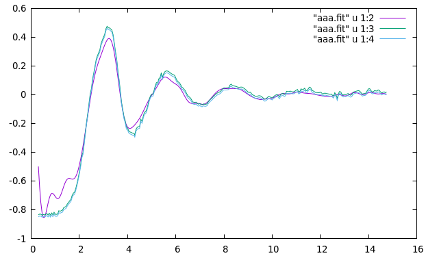
Figure: Comparison of the S(Q) of an RMC structural model with experimental S(Q). Two experimental curves are shown because one is corrected.
For the underlying convention, see equation (E3) and its surrounding discussion in the user guide.
.hst: Chi-squared history and fit progress
This file contains History data produced by History::save
:
:
For F(Q) data set 1	F(Q) fitting was used

generated       	tried           	accepted        	time      	tried/gen       	acc/tried       	chi2_tot/data_point;       	chi2/F(Q)_set#1;
               0	               0	               0	         0	        0.000000	        0.000000	1.578930954817895e+02      	4.578899768971894e+04
              30	              17	              11	         0	        0.566667	        0.647059	1.574103409681942e+02      	4.564899888077633e+04
              77	              39	              22	         0	        0.468085	        0.500000	1.569245983657412e+02      	4.550813352606496e+04
             113	              62	              33	         0	        0.638889	        0.478261	1.567761016798288e+02      	4.546506948715034e+04
             146	              80	              44	         0	        0.545455	        0.611111	1.563252734257866e+02      	4.533432929347811e+04
             163	              91	              55	         1	        0.647059	        1.000000	1.562772215647136e+02      	4.532039425376695e+04
             211	             116	              66	         1	        0.520833	        0.440000	1.560415962591003e+02      	4.525206291513910e+04
             249	             142	              77	         1	        0.684211	        0.423077	1.557480271250309e+02      	4.516692786625896e+04
         :
         :
           61999	           36721	            9713	       119	        0.575342	        0.261905	1.117579568397242e+02      	3.240980748352001e+04
           62010	           36729	            9715	       120	        0.727273	        0.250000	1.117680889621432e+02      	3.241274579902153e+04

The Rw values for the data sets are:
          F(Q) set #1	 1.755480e+01

The calculation method for the chi_square/data sets

   1 F(Q) data series :   normal
This file shows how the fit changes as RMC steps accumulate. The seventh column, chi2_tot/data_point, is the total χ² normalized per data point. The eighth column, chi2/F(Q)_set#1, is the χ² for F(Q) dataset 1. Do not confuse total χ² with χ² per data point.
Plotting the history reveals whether the metric decreases with increasing steps, indicating improvement in the fit. Convergence should be assessed not only by whether χ² has become sufficiently small, but also by inspecting the actual S(Q) curves and the partial pair-correlation functions gᵢⱼ(r).
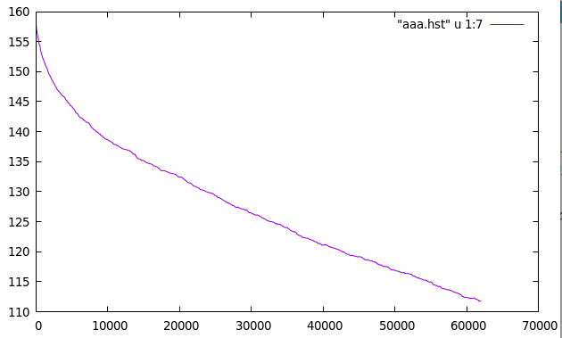
Figure: Evolution of chi2_tot/data_point.
Partial pair-correlation functions gᵢⱼ(r)
Example: aaa.ppcf
This is an object of Class PPCFSet
3	 number of atom types

For data set(s) 1
306	 number of discretization bins for the ppcf
0.000000000	 rmin value (Angstroms)
7.650000000	 rmax value (Angstroms)
0.025000000	 discretization step (Angstroms)

r value + 6 partial g(r) at the middle of the histogram bin
0.012500000	         0.000000000	         0.000000000	         0.000000000	         0.000000000	         0.000000000	         0.000000000
0.037500000	         0.000000000	         0.000000000	         0.000000000	         0.000000000	         0.000000000	         0.000000000
0.062500000	         0.000000000	         0.000000000	         0.000000000	         0.000000000	         0.000000000	         0.000000000
0.087500000	         0.000000000	         0.000000000	         0.000000000	         0.000000000	         0.000000000	         0.000000000
0.112500000	         0.000000000	         0.000000000	         0.000000000	         0.000000000
    :                    :                   :                   :                   :                   :
This file contains the calculated partial pair-correlation functions gᵢⱼ(r). Starting at line 11 of this example, the columns give r and the functions for each atomic-species pair. With three species there are six distinct pairs, so the column order is:
r [Å], g11(r), g12(r), g13(r), g22(r), g23(r), g33(r).
See the final line of section B of the user guide.
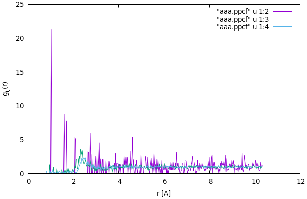
Figure: Examples of g11(r), g12(r), and g13(r).
Atomic configurations and three-dimensional visualization
Example: aaa.cfg
The output configuration uses the same format as the input .cfg file. It is overwritten as the simulation continues. Convert it as appropriate for visualization with VESTA, OVITO, or another structural viewer.
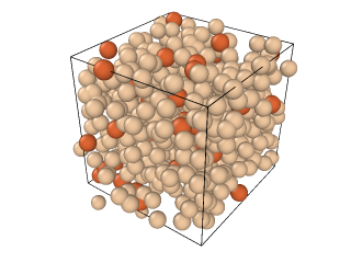
Figure: Example of a structure obtained through RMC_DFT.