Fundamentals of Choosing a First-Principles Calculation Code

K. NAKADA
This article was written around November 2015, at the request of CMSI, as an introduction to first-principles calculations for beginners. In the end, however, I never submitted it to CMSI. There is a bit of a story behind it: just before submitting the final manuscript, I had to withdraw at the last minute because of circumstances related to my position at the time. I caused considerable inconvenience to the professors who reviewed the manuscript and to everyone else involved, for which I apologize. Since it seemed a shame to leave the manuscript buried in my archives, I dug it out, converted it to Markdown, and decided to make it public.

• Fundamentals of Choosing a First-Principles Calculation Code
  • Introduction
  • First-Principles Methods Based on DFT Solve the KS Equation (a Kind of Schrödinger Equation)
    • (1) Four Factors Directly Responsible for Differences Among Calculation Codes
    • (2) Shape of the Potential and Treatment of Core Electrons
    • (3) Representation of Solids
    • (4) Choice of Basis Functions
  • Choice of Basis Functions
    • (1) Localized Basis Functions
    • (2) Plane-Wave Basis Functions
      • (2)-(A) All-Electron Calculation Methods
      • (2)-(B) Pseudopotential Methods
      • (2)-(C) The PAW Method
  • A Summary of First-Principles Calculation Codes Classified by Basis Functions
  • First-Principles Calculation Codes Around the World
  • Physical Quantities That Can Be Calculated with Any Code
  • Can a Code Calculate a Particular Physical Quantity? Codes Capable of Calculating XANES Spectra
  • Calculating Other Physical Quantities and Interfacing with Other Codes
  • The Popularity of Calculation Codes
  • Summary of Calculation Codes

Introduction

CMSI’s MateriApp introduces a wide variety of first-principles calculation codes, including Akai-KKR, OpenMX, xTAPP, and ABINIT. People attempting such calculations for the first time often find themselves bewildered by the differences among these codes.

Understanding those differences in depth normally takes a great deal of time. Nevertheless, by keeping a few key points in mind, even someone who is not a specialist in computational physics can gain a reasonably sound understanding of how the codes differ. This document is intended to help nonspecialists grasp, in broad terms, the differences among calculation codes and the methods they employ. I hope it will be useful to experimentalists and researchers working in industry.

Much of this document is a written version of part of a lecture I gave on July 28, 2015, at the “First Workshop on Computational Science for Materials Structure Analysis at SPring-8.” A publicly available version of the original presentation slides can be found on the SPring-8 website. (If that link no longer works, try this link, accessible only within the SPring-8 site.)

Specialists may find the discussion excessively rough, or may even feel that some of what I say is rather careless. In fact, my own specialty is the FLAPW method, which places me somewhat apart from the mainstream, so my knowledge is decidedly skewed. I have also been away from active code development and related work for quite some time. On top of that, the discussion probably contains a fair amount of my own arbitrary judgments and biases. Needless to say, there are limitations both in my knowledge and in my ability to communicate it. I would encourage specialists to consult specialist textbooks instead. Above all, the material was originally prepared for a 20-minute presentation, so I proceed in a fairly broad-brush, informal fashion; the intended audience, after all, is beginners. I ask for your understanding on that point.

Unfortunately, there is no universal calculation method—or calculation code. If this document helps more people recognize the distinctive characteristics of different codes and choose among them according to the problem they need to solve, it will have served its purpose.

First-Principles Methods Based on DFT Solve the KS Equation (a Kind of Schrödinger Equation)

What equation do first-principles calculations based on density functional theory (DFT) actually solve? I think the simplest answer is that they solve the Kohn–Sham (KS) equation.

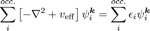
For most purposes, it is perfectly reasonable to think of this equation as “the Schrödinger equation for a single electron in an effective potential.” The differences among calculation codes lie in how they solve this equation. The reason codes around the world are so diverse is that they differ in which approximations they apply to the various elements making up the KS equation, and in how they then solve it. Each approach has its strengths and weaknesses. Before attempting a systematic comparison of the codes, I would like to explain these components briefly.

These components remain fundamentally important even when one adopts approximations or approaches that go beyond the DFT–KS equation¹. It is therefore worth understanding the following points.

(1) Four Factors Directly Responsible for Differences Among Calculation Codes

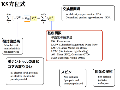
As the atoms under consideration become heavier, relativistic effects can no longer be ignored. There are several levels of approximation, but most first-principles calculations employ the scalar-relativistic (or semi-relativistic) approximation, which includes relativistic effects other than spin–orbit coupling. It is worth remembering that scalar-relativistic treatment is, at the very least, essential once the atomic number exceeds 30. Caution is also called for above atomic number 20.

Some quantum-chemistry DFT codes, which often deal primarily with light elements, deliberately default to a nonrelativistic treatment without even including scalar-relativistic effects. Care is therefore needed when using such codes for 3d transition metals.

As you probably know, relativistic effects including spin–orbit coupling play an important role in heavy elements, including rare-earth elements. In first-principles calculations, however, there are several different schools of thought—or approximations—for introducing spin–orbit coupling.

Broadly speaking, a treatment combining scalar relativity and spin–orbit coupling is called fully relativistic. In practice, however, the mainstream approach is to introduce “scalar relativity + spin–orbit coupling” through what is known as the second-variational method². This makes full-potential calculations possible at a practical computational cost and within a reasonable level of approximation. Of course, some codes incorporate relativistic effects using more sophisticated approximations, although these are usually computationally more expensive.

I will not go into the details of how relativistic effects, including spin–orbit coupling, are treated in first-principles calculations here. It is important, however, to exercise care when spin–orbit coupling is essential to the physical properties being investigated.

(2) Shape of the Potential and Treatment of Core Electrons

Let us consider the approximations made to the shape of the potential when solving the KS equation. There are two major approaches: the muffin-tin (MT) approximation, which assumes spherical symmetry, and the full-potential approach, which does not impose such a restriction on the shape of the potential.

Naturally, a full-potential treatment is a better approximation than the MT approximation. However, the MT approximation works well, for example, in densely packed metallic systems, and allows problems to be solved very quickly (and with low memory consumption). It would therefore be wrong to dismiss it categorically as a poor approximation.

Many mainstream codes today use full-potential approaches without users having to give the distinction much thought. Nevertheless, there are still many computational methods that, because of how they treat relativistic effects or because of issues involving basis functions discussed later, must solve problems within the MT approximation³. It is also worth remembering that the MT approximation is often perfectly adequate for the material system being studied. Each approach has advantages and disadvantages, which we will summarize later.

For surfaces and molecules, of course, the MT approximation is generally not very good. For such systems, it is preferable to use a full-potential method wherever possible⁴.

Codes based on the pseudopotential method, which forms the mainstream of first-principles calculations, are also full-potential as far as the shape of the potential is concerned. The trade-off is that conventional pseudopotential methods do not explicitly calculate the electronic states of core electrons, and this limitation must be kept in mind.

(3) Representation of Solids

Although this is closely tied to the choice of basis functions discussed later, methods can broadly be divided into those that calculate using periodic unit cells and those that treat isolated molecules or atoms. There are also real-space methods, but these are a fairly small minority among widely used first-principles codes, so I will omit them here. I will return to this distinction in somewhat greater detail when discussing the choice of basis functions in a later section.

(4) Choice of Basis Functions

Most first-principles calculation codes solve the KS equation by expanding the relevant quantities in basis functions. Some codes instead divide space into a mesh and solve the KS equation as a second-order partial differential equation using a real-space finite-difference formulation (FDM). Such approaches, however, are relatively uncommon⁵.

In most calculations, the wavefunctions are expanded in basis functions and the resulting equations are solved. Consequently, every component of the KS equation is closely related to the choice of basis functions. Naturally, it is not only the wavefunctions that are expanded: the electron density and potential are also represented using basis functions.

For this reason, understanding the characteristics of the basis functions is, in most cases, enough to understand the essential characteristics of a calculation code. I will discuss this in more detail in the next section.

Equation

Choice of Basis Functions

There are two broad approaches to choosing basis functions. One uses localized basis functions (local bases); the other uses plane-wave basis functions.

(1) Localized Basis Functions

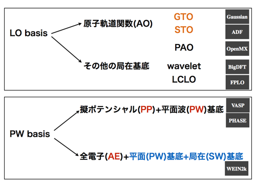
When dealing with atoms and molecules, functions localized around individual atoms provide a more natural representation of their one-electron states. In many cases, one chooses atomic orbitals or basis functions constructed from their linear combinations (LCAO). For example, codes such as Gaussian solve the KS equation using Slater-type orbitals (STOs) or Gaussian-type orbitals (GTOs) as atomic basis functions, making it particularly straightforward to describe the electronic states of atoms and molecules.

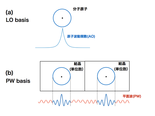
There are various advantages to this choice of basis, but one of the most significant in practice is that the number of basis functions is extremely small compared with a plane-wave expansion. In other words, calculations are dramatically less demanding—and faster. Memory requirements are also lower. Furthermore, because the starting point is a wavefunction localized around an atom, this representation is close to the physical picture used in model-based descriptions. It is therefore particularly well suited to analysis and interpretation in terms of such pictures. For example, many types of bonding analysis become relatively easy, among numerous other analytical advantages.

Of course, there are also plenty of disadvantages. Many basis sets built from STOs or GTOs do not form a complete basis⁶. Superposing STOs or GTOs alone cannot describe the system’s one-electron states perfectly: some incompleteness remains. Because one is using a localized and incomplete basis set, an additional term known as the Pulay correction appears when calculating the forces acting on atoms. Force calculations are consequently troublesome, and molecular dynamics in particular is considerably less convenient than with a conventional plane-wave basis. There are further computational complications, such as the need to account for basis-set superposition error (BSSE), arising from overlap between localized wavefunctions. This is another reason why molecular dynamics is difficult with these approaches.

Moreover, for systems involving d orbitals, a simple basis set often fails to provide an adequate description. One must select a suitable basis set for each material under study, and doing so often requires experience⁷. Closely related difficulties may also arise in achieving convergence. Conversely, with sufficient experience, if one can calculate the molecule of interest using the minimum necessary basis set, it is possible to obtain reasonably good results remarkably quickly.

Another advantage is that methods using localized basis functions can readily perform so-called all-electron calculations, including the electronic states of core electrons⁸. This also makes it relatively easy to calculate spectra involving core-level excitations, such as X-ray absorption fine structure.

These methods are also not particularly well suited to calculations on solids with periodic unit cells, which I discuss in the next section. To begin with, STO and GTO basis functions do not, in any straightforward way, form the Bloch functions needed to describe one-electron states in crystals. However, even among methods derived from localized bases, there are of course approaches that construct the expansion to have Bloch-function form from the outset. These include the early cell method and methods such as KKR and LMTO. Such approaches are well suited to periodic solids but, conversely, less suited to molecular systems. I will not pursue the details here, as they would complicate the discussion. For the purposes of the present discussion, please understand “localized basis” as referring mainly to STO- and GTO-based approaches commonly used in quantum chemistry.

(2) Plane-Wave Basis Functions

For materials such as solids with periodic boundary conditions, the one-electron states in a crystal must take the form of Bloch functions. A plane-wave (PW) basis makes such states extremely easy to describe. Conversely, a plane-wave code cannot directly treat a nonperiodic system without some additional device. For molecular calculations, for instance, one must construct a cell containing a sufficiently large vacuum region. Similarly, to model a surface—where periodicity is broken in one direction—one generally constructs a periodically repeated slab separated by vacuum.

A further problem is that, if one makes the unit cell large enough for part of it to be regarded as vacuum, the plane waves still extend throughout the entire cell. As the cell grows, more and more plane waves are needed, and the computational cost rises steeply with the volume. In a conventional plane-wave treatment, basis functions are needed even in the vacuum region. In this sense, plane-wave methods are not particularly good at molecular or surface calculations. Such calculations are certainly possible, but it is worth remembering that the fundamental strength of the approach lies in systems with periodic boundary conditions.

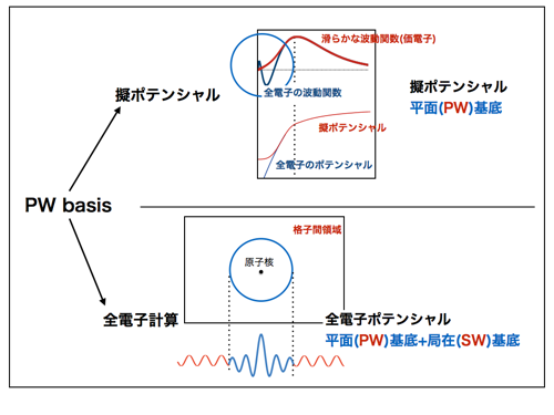
This may sound contradictory to what I have just said, but there is another important point: a simple plane-wave basis by itself cannot realistically handle a crystal while also describing its core states. If plane waves alone were enough, nobody would have had to struggle with this problem. In real crystals, electronic states change extremely rapidly near atomic nuclei. With localized basis functions, wavefunctions that vary sharply near the nucleus can be represented directly at relatively low cost. Reproducing those same rapid, localized variations with plane waves, however, would require an enormous number of basis functions; achieving convergence becomes prohibitively difficult in practice. Thus a straightforward plane-wave expansion is not, by itself, a practical solution for crystalline electronic structure.

A variety of methods have therefore been developed starting from the plane-wave basis. Naturally, methods built on plane waves share the basic characteristics outlined above. Setting aside their historical development and finer details⁹, I will now give a broad, informal explanation of two approaches that can be regarded as mainstream today.

(2)-(A) All-Electron Calculation Methods

A distinctive feature of electronic states in solids is that they have two very different characters at once. In the regions between atoms—the interstitial (IT) regions—the electronic states vary relatively smoothly and are easily described by plane waves. Near the nuclei, on the other hand, the states vary rapidly and are better described by localized basis functions. Methods were therefore devised that combine these two different descriptions: localized functions near nuclei and plane waves in the interstitial regions¹⁰.

Because localized functions can be expressed through the spherical-wave expansion of plane waves, the underlying idea is still essentially plane-wave-based: augment the plane waves only in the vicinity of the atomic nuclei. The crystal potential and wavefunctions are then represented using this augmented construction. This is the family of methods developed under the names APW, LAPW, and FLAPW. Roughly speaking, you can think of the basis as a combination of plane waves (PWs) and spherical waves (SWs). Codes employing these methods include WIEN2k, exciting, FLEUR, HiLAPW, ABCAP, and KANSAI. Their defining characteristic is that they describe the electronic states of solids head-on, without sidestepping the core-electron problem.

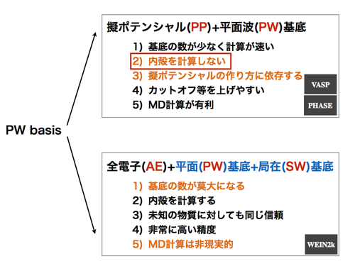
Because the core-electron states are calculated afresh each time to construct the crystal potential, these methods can deliver highly accurate calculations even for previously unknown materials. Since the calculation starts from the atomic core states, in principle the only atomic information one needs to supply is the atomic number. The earliest implementations used the muffin-tin (spherically symmetric) approximation, but M. Weinert subsequently developed the full-potential method. Today, practically all methods in this family are full-potential methods, with no assumption imposed on the shape of the potential.

These all-electron methods may sound universally applicable, but their greatest drawback is the enormous number of basis functions and the resulting computational cost. Augmenting plane waves also raises the issue of overcompleteness, and there are difficulties in calculating atomic forces that resemble, in a certain sense, those encountered with localized bases. In other words, these methods are simply not suited to molecular dynamics. To begin with, the basis is huge and the calculations are far too expensive.

FLAPW has a number of more subtle problems as well, including fundamental issues associated with linearized band calculations¹¹. Nevertheless, in terms of reliability and the ability to tackle unknown materials, it serves as a benchmark for virtually every other calculation method. When people say that a code has “good accuracy,” what they usually mean is that its results differ little from those obtained with an FLAPW code such as WIEN2k.

Furthermore, because these methods properly calculate the core states, they can relatively easily calculate X-ray absorption fine structure¹² and often obtain quite good agreement with experiment. At the same time, because they are fundamentally plane-wave-based methods built around periodic boundary conditions, the caveats about molecules and surfaces discussed above still apply. In particular, FLAPW requires so many basis functions that filling a vacuum region with the same enormous basis makes calculations on molecules and surfaces almost absurdly expensive. Frankly, I find it difficult to recommend FLAPW for such systems.

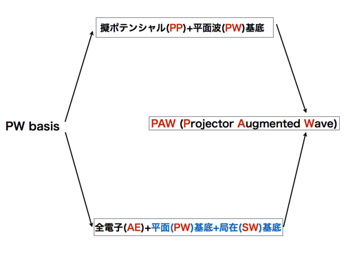
(2)-(B) Pseudopotential Methods

Another family of plane-wave-based first-principles methods, besides all-electron methods, is the pseudopotential method. Broadly speaking, pseudopotential methods rest on two basic ideas. The first is to treat the core-electron problem as a core-electron problem and the valence-electron problem as a valence-electron problem: it is sufficient to solve the latter correctly. Thus, whether we calculate TiO2 or TiN, for example, the core-electron states of Ti are treated as those of Ti. This is the approximation known as the frozen-core approximation.

The second idea is to use an artificially constructed pseudopotential that reproduces the results obtained with the true valence electrons. The problem can then be solved in terms of a smooth pseudopotential and its corresponding pseudo-wavefunctions, which can be represented with a manageable number of plane waves. Although we are solving a problem involving pseudopotentials and pseudo-wavefunctions, an appropriately chosen pseudopotential gives the same results as a calculation using the true valence-electron states. In practice, pseudopotentials are constructed to reproduce results from all-electron methods such as WIEN2k. In principle, therefore, it is possible to obtain results with accuracy comparable to all-electron calculations.

The greatest advantage of pseudopotential methods is that, by preparing a sufficiently smooth pseudopotential, the number of plane waves (basis functions) required can be made extremely small. Calculations are overwhelmingly faster than with all-electron methods. Moreover, because the forces acting on atoms can readily be evaluated using the complete plane-wave basis, molecular dynamics calculations can be performed both accurately and rapidly. This is a major advantage over other calculation methods.

There is another benefit: unlike all-electron calculations, the basis is not so extravagantly large to begin with, so it is relatively easy to increase the number of plane waves—that is, to raise the cutoff. In contrast to all-electron methods such as FLAPW, where an already lavish basis makes further increases difficult, one can keep cranking up the cutoff, thereby increasing the variational freedom available to the calculation.

The drawback is that the results depend strongly on how the pseudopotential is constructed. For an unknown material, there is no guarantee that a given pseudopotential is truly appropriate. In a sense, one might even say that the reliability of a calculation code is directly tied to the reliability of the pseudopotentials its developers have painstakingly constructed. Furthermore, because the core-electron states are not recalculated each time, such methods naturally cannot calculate excitation spectra originating from core states, such as X-ray absorption fine structure¹³. They do not possess the information about the true crystal potential, including the core, or the true wavefunctions.

Historically, the basic idea behind pseudopotential methods developed gradually from the OPW method¹⁴. It subsequently underwent major advances, including the norm-conserving pseudopotential (NCPP) method, which constructs pseudopotentials from first principles, and the ultrasoft pseudopotential (USPP) method, which achieves smoother pseudopotentials by ensuring conservation of the charge as viewed from outside rather than enforcing norm conservation. Nevertheless, the essential characteristics remain those described above. I will omit the individual properties and technical details of these different pseudopotential methods here¹⁵.

(2)-(C) The PAW Method

Pseudopotential methods made it possible to achieve quite high accuracy with relatively few plane-wave basis functions. Nevertheless, they have difficulties describing electronic properties associated with regions close to the core: for example, d orbitals involved in magnetism, which are relatively localized around atoms; core states becoming part of the valence states under high pressure; and the accurate treatment of shallow core states¹⁶.

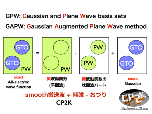
To address problems in which these core-related electronic states are important, a method was devised to incorporate into pseudopotential calculations the treatment of electronic states near the core used in all-electron methods. This is PAW (the Projector Augmented Wave method). In PAW, projectors map pseudo-wavefunctions onto all-electron wavefunctions. Thus, although the actual calculation solves a pseudopotential problem using pseudo-wavefunctions, it can yield the same answer as an all-electron problem. Perhaps the easiest way to express the idea, in deliberately simplified terms, is “all-electron = pseudopotential calculation + core calculation − a compensation term.” Consequently, subject to the restriction that the supplied pseudopotential is frozen¹⁷, pseudopotential-based calculations can attain accuracy comparable to FLAPW.

The idea can also be viewed as essentially the same as that underlying the SW-LAPW basis, developed as a formalism that permits force calculations with an LAPW basis: “a smooth wavefunction defined throughout space + localized orbitals − a compensation term”¹⁸. Seen in this light, the subsequently developed PMT (augmented Plane Wave and Muffin-Tin orbital) method can be understood as introducing smooth, Hankel-function-type localized basis functions in addition to plane waves as the carrier basis¹⁹.

There is also a method called GPW (Gaussian and Plane Waves), used in the CP2K code, which can be understood here in relation to the ideas behind PAW. Rather than using spherical waves for the atomic-site augmentation, it uses GTOs. This approach also addresses one of the major weaknesses traditionally associated with GTO-based codes: their relative unsuitability for molecular dynamics. In other words, one can think of it as reinforcing plane waves with Gaussians. In practice, the problem is solved at the level of a plane-wave-based pseudopotential calculation, while GTOs provide augmentation for electronic states near the cores.

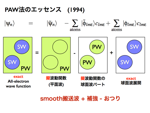
Such calculations therefore require pseudopotentials. In recent years, basis functions derived from ideas such as PAW, together with their extensions, have become increasingly common, gradually overcoming the weaknesses of conventional basis sets. At first glance these methods may appear completely different, but if one keeps the basic idea of PAW in mind, I think they can be sorted into broad categories fairly easily. One expression I use repeatedly in this document is PP-PAW for the PAW method employed in codes such as VASP, since it is PAW based on a pseudopotential (a smooth plane-wave basis). This is not merely notation of my own invention; although a little specialized, it is reasonably common.

A Summary of First-Principles Calculation Codes Classified by Basis Functions

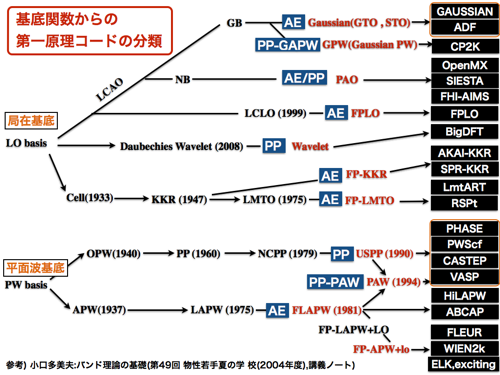
I would like to briefly summarize the discussion so far. In most cases, I think the knowledge covered up to this point should be enough to organize the various codes and compare them systematically. Throughout this document, AE generally means all-electron: in other words, the electronic states of the core electrons are explicitly calculated. For example, FLAPW is an all-electron method, so I sometimes deliberately write AE-FLAPW here, although this notation is hardly conventional²⁰. Similarly, I deliberately write AE-GTO, even though people normally would not: one might say that FLAPW and GTO are all-electron methods as a matter of course. I use these labels here solely to make the classification unambiguous.

As mentioned earlier, I write PP-PAW for the pseudopotential-based PAW method²¹. The name ultrasoft pseudopotential (USPP) already contains PP, yet I sometimes insist on writing PP-USPP as well. Nobody normally does this. For a rather specialized—or perhaps downright obscure?—basis such as wavelets, readers unfamiliar with the method may not know whether it uses pseudopotentials or treats all electrons. In that case, PP-Wavelet seems a helpful label, although I have never actually seen anyone use it. Likewise, OpenMX and SIESTA, which use numerical localized basis functions (PAOs or NBs), a family of localized bases I did not explain in detail here, are labeled PP-PAO. This notation is relatively common. In contrast, FHI-aims also uses numerical basis functions but performs all-electron calculations, so I call it AE-PAO; I do not think this terminology is widely used.

The labels in this classification reflect my own personal judgments and preferences, so I recommend that you not use them too freely in public. I have also omitted FDMNES and RSPACE, mentioned in the main text or footnotes, because they are not based on basis-function expansions. I apologize for leaving out ecalj, which uses the PMT method: there simply was not room in the table. For the same reason, I have omitted the mountains of other codes available worldwide, particularly pseudopotential-based ones.

Another topic I barely discussed, mainly to keep the narrative manageable, is the KKR Green’s-function method. It remains an important computational method today, not least for practical reasons. To understand it properly, comparing APW with KKR and LAPW with LMTO is, if anything, essential and unavoidable. This time, however, trying to weave KKR into the same explanatory story would have made it excessively long and complicated, so I left it out for convenience. I hope to return to it on another occasion, with a different organization of the material.

From a practical standpoint, the KKR method developed under the muffin-tin (MT) approximation, but full-potential formulations now exist. As far as I know, however, there is currently no publicly released full-potential KKR code in a form that ordinary users can readily employ. The publicly available versions of AKAI-KKR and SPR-KKR remain within the MT approximation, so care is needed when choosing the systems to which they are applied. On the other hand, precisely because KKR is a Green’s-function method, incorporating the coherent potential approximation (CPA) is straightforward, making it extraordinarily powerful for calculations on alloys and related systems.

The LMTO method, which can be viewed as a linearized form of KKR, is astonishingly fast: when performing calculations of roughly the same level as LAPW within the MT approximation, it requires a remarkably small number of basis functions. However, like the MT-based KKR Green’s-function method, it does not give particularly good results for systems with low packing fractions. Even in such systems, results can be improved to some extent by introducing fictitious atoms with atomic number zero, known as empty spheres (ES). Their placement, however, involves arbitrary choices and therefore requires experience.

FP-LMTO, the full-potential version intended to overcome these limitations of the MT approximation, ultimately achieves roughly the same accuracy as FLAPW at roughly the same computational cost. Consequently, it has not become especially widespread in practice (FLAPW was already available and could do essentially the same job). There are surely many other practically important points and calculation codes that deserve mention, and some readers may disagree with my choices. For the purposes of this document, however, I have grouped the codes as shown on the preceding page.

Above all, I have tried to include representative codes. Naturally, my own tastes have also influenced the selection. Because of space limitations, I have listed only Gaussian and ADF among quantum-chemistry codes. In fact, given the size of the quantum-chemistry community, I suspect that localized-basis DFT codes developed there constitute the largest group of DFT codes in terms of the number of programs under development. They are actually the biggest contingent. Many readers probably use them, but I will say very little about them here.

First-Principles Calculation Codes Around the World

By now, I think we have acquired enough background to understand the fundamental differences among calculation codes, particularly those arising from their choice of basis functions. With that in mind, let us first look at Wikipedia’s list of first-principles calculation codes.

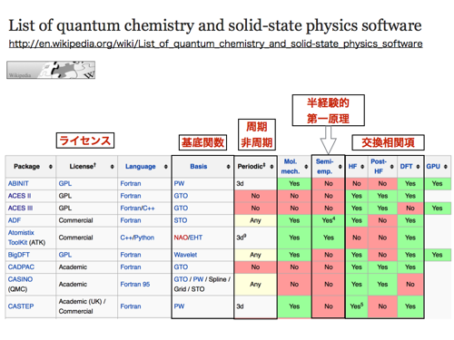
Some entries look a little questionable, but the table provides information such as the basis functions employed and whether each code handles periodic or nonperiodic systems. This makes the classification remarkably easy to follow. Once you understand the basic distinctions among basis functions, you can more or less infer the characteristics of a code. For example, as discussed above, codes using localized basis functions—GTOs or STOs—are usually intended for nonperiodic systems. Broadly speaking, you can think of these as codes for molecular calculations. They have mainly been developed within the quantum-chemistry community. Of course, some codes using localized bases can also calculate periodic systems.

Conversely, when the basis consists of plane waves (PW), the starting assumption is a periodic system (marked “3d” in the table). These codes have mainly been developed in the physics community and are particularly well suited to bulk calculations. With PW bases, one can also devise suitable periodic models, such as periodic slab models, to calculate molecules and surfaces at fairly reasonable computational cost and accuracy.

The exchange–correlation entry, meanwhile, concerns the approximation used in calculating the potential. This is important, but I have deliberately avoided explaining it here, because doing so would derail the discussion. For the moment, if you see “DFT,” just take it to mean an ordinary first-principles calculation. Think of HF as a method that treats the exchange term exactly, and post-HF as methods that go beyond this by improving the treatment of correlation as well. These methods are not necessarily superior to DFT across the board. Semi-empirical methods include empirical parameters, so I would suggest that beginners steer clear of them for the time being.

In actual practice, however, the license category may well be the most important distinction of all. This deserves careful attention. As you know, the GPL is a license commonly used for open-source software. You can use GPL-licensed codes for calculations free of charge, and they can generally be downloaded directly. Naturally, if you modify GPL-licensed code or reuse its source, you must comply with the GPL’s terms.

Codes classified as “Academic” often have their own licenses, in many cases rather loosely based on licenses such as MIT/X11, but you must check the terms of each individual license. They are frequently intended primarily for use at universities and other research institutions. Moreover, obtaining an academic code often requires emailing its author or registering your email address, affiliation, and other details on a website. Particular care is needed if you intend to use one in a company.

Another point to keep in mind is that many of these first-principles codes are written in Fortran. Occasionally a code is described as being written in C, but a particular solver may actually be written in Fortran, in which case a Fortran compiler is also required.

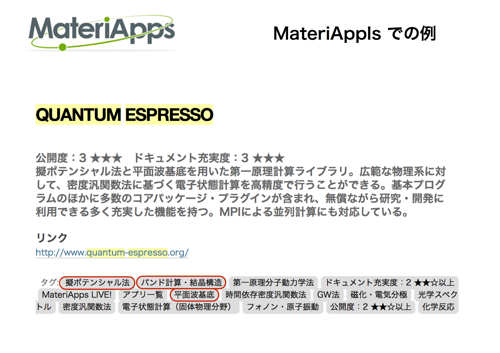
Thus, although Wikipedia’s page offers relatively little detail because it is organized as a table, I think it provides an excellent overview of the important differences among codes. There are also introductions prepared by specialists, rather than pages on Wikipedia whose reliability can sometimes be anyone’s guess. Such resources may list fewer codes than Wikipedia (or sometimes more). One example is CMSI’s MateriApps, which also introduces computational codes. If you know terms such as “pseudopotential method,” as explained in this document, MateriApps becomes an excellent source of information. Its descriptions of the codes are carefully prepared. Browsing through them can lead you to discover some extremely useful programs, so I encourage you to explore the site.

Physical Quantities That Can Be Calculated with Any Code

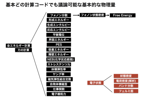
By now, I think you have seen just how many calculation codes there are around the world. If you are using one for the first time, however, deciding which one to choose can be quite bewildering. As I explained earlier, different basis sets make different codes better or worse suited to particular classes of materials. Leaving that aside, though, virtually any of these codes can perform the basic calculations of electronic structure. There are an enormous number of codes based on plane waves (PW), in particular, and to a considerable extent they can all do much the same work. For example, simply being able to obtain the total energy of a given structure already makes it possible to calculate or discuss the remarkably wide range of physical quantities shown in the figure below. And, since these are electronic-structure calculations, quantities such as wavefunctions and charge densities are already being calculated; local densities of states, band dispersions, and Fermi surfaces can therefore also be obtained with any of these codes. Does that mean the choice of code makes absolutely no difference? Of course not. There are subtle differences. Quite apart from the approximations employed, there is also the question of how mature and well-developed each code is²².

Can a Code Calculate a Particular Physical Quantity? Codes Capable of Calculating XANES Spectra

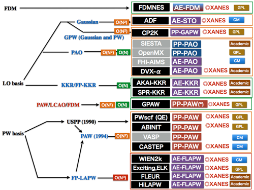
As I have rather insistently pointed out in the footnotes and elsewhere, calculating X-ray absorption fine structure naturally requires a treatment of core electrons. In most cases, this means using a method based on localized STO or GTO basis functions, or the FLAPW method. Calculations are also possible with PP-PAW methods and GPAW. Likewise, all-electron methods based on KKR can, of course, calculate XANES. In fact, within the XAFS community, the mainstream approach to calculating XANES and EXAFS is to use codes based on multiple-scattering theory formulated in terms of Green’s functions.

The following figure is my attempt to summarize the major codes capable of calculating XANES (along with a few codes that cannot, but which I included anyway because they seemed to belong in the classification). It is almost the same table as the earlier classification by basis functions, except that the emphasis here is specifically on whether each code can calculate XANES. I have also included codes that calculate XANES spectra using the finite-difference method (FDM), which I have barely discussed in this article. Some codes, such as GPAW, support several representations or methods, including FDM, linear combinations of atomic orbitals (LCAO), and plane waves (PW).

One point that deserves particular attention when choosing a code for actual research is whether it can calculate the L absorption edges. For example, at least in their publicly available versions, CP2K, GPAW, and Quantum ESPRESSO cannot calculate L-edge spectra. If you need L-edge calculations, you must turn to an FLAPW code such as WIEN2k or to commercial software such as CASTEP. VASP, which is in practice very similar to CASTEP, cannot at present calculate XANES at all, let alone the L edges²³. In this respect, for bulk systems, WIEN2k can calculate XANES including the L edges, even if the calculations are computationally expensive. For molecular or surface systems, however, codes that can calculate spectra all the way through the L edges may appear to offer several options, but in practice there are very few²⁴.

Calculating Other Physical Quantities and Interfacing with Other Codes

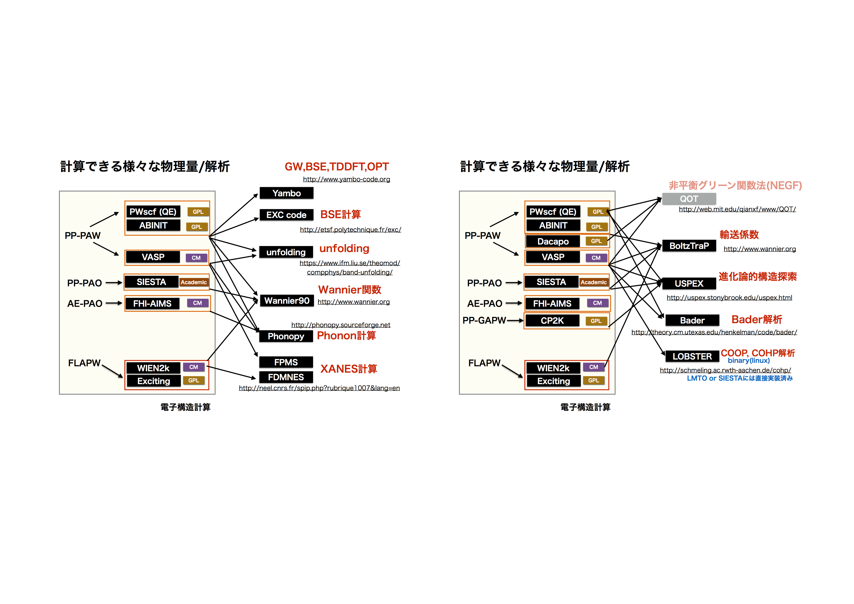
Because XANES calculations require the electronic states of core electrons, the choice of calculation code becomes considerably more restricted²⁵. There are other limitations as well. For example, charge-population analyses such as Mulliken analysis, which are based on localized wavefunctions, cannot be performed directly with a plane-wave basis. In recent years, however, real-space charge-density analysis, notably Bader analysis, has advanced to the point where even plane-wave calculations can be analyzed using charge densities on a real-space mesh²⁶. Similarly, bonding analyses such as COHP, originally associated with localized basis sets, can now be carried out much more widely for plane-wave calculations through methods such as projected COHP (pCOHP), which projects the electronic states onto specified orbital components of particular atoms.

Sometimes these capabilities are included in the calculation package itself. Quite often, however, a separate analysis program reads the electronic states obtained from the original calculation and analyzes them afterward. The Japanese plane-wave code PHASE, developed in connection with national research projects, comes with a package capable of calculating many physical quantities, including dielectric functions. Fundamentally, though, these analyses use results calculated by PHASE. More recently, as many calculation codes have become open source under licenses such as the GPL, it has increasingly become possible to link numerous programs together. Consequently, electronic-structure calculations and the subsequent evaluation of physical quantities are more often performed by different codes. This means that, for the basic electronic-structure calculation, you can use a familiar code suited to the material system you want to study.

I have not mentioned this explicitly so far, but many codes developed overseas have also made considerable progress in modularizing their fundamental computational components—for example, solvers for electron correlation and eigensolvers for large-scale calculations. In the past, an individual research group would independently implement virtually every solver needed for its calculations. More recently, many codes have been developed in a more open-source-oriented manner, and an increasing number of their components are becoming shared modules.

Of course, moving back and forth among different codes and approximations carries risks. It becomes harder to see where the essential problem lies, and blindly combining incompatible approximations is dangerous. Nevertheless, even though the subject is physics, a calculation code is still a computer program. With source-code distribution under the GPL becoming more common, I think we are gradually beginning to see a change in the way these codes are developed: work based on the same underlying theory is increasingly shared rather than independently reimplemented.

The Popularity of Calculation Codes

So far, we have looked at a variety of calculation codes, classified them by their basis sets, and discussed the kinds of material systems for which they are best suited. We have also seen that some physical quantities can only be calculated with particular codes, although the growing ability of different programs to work together means that it is sometimes possible to obtain those quantities through a separate post-processing calculation. In practice, however, perhaps the single biggest factor in a user’s choice of code is its popularity—its share of the user community.

Widely used codes have much more information available about them. Because so many people use them, bugs are actively fixed, discussions are plentiful, and users’ requests are more likely to be addressed. Unless there is some special requirement such as “Only this code can calculate the particular physical quantity I need!”, I suspect most users do not demand all that many things of a calculation code. Their requirements may boil down to three: “It converges well,” “It runs fast,” and “Its results are reliable.” There are plenty of excellent, less widely used codes. Still, the most popular codes generally have good reasons for being popular, and they really are quite capable.

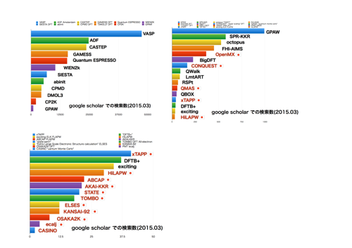
And once a code wins the battle for popularity, the one with the largest share eventually becomes the established standard. You may have some objections to my choice of codes and search keywords, but the figure below shows the numbers of papers found by searching Google Scholar. I have excluded quantum-chemistry codes. One reason is that a name such as Gaussian is so general that it is difficult to isolate papers referring specifically to the Gaussian program. Even with the search narrowed down, however, the number of papers is more than an order of magnitude greater than that for VASP, the largest entry in the figure. Considering the relative sizes of the chemistry and physics communities, that may be only natural. I have also excluded PHASE, which I mentioned briefly earlier: its name is so common that narrowing the search sufficiently was difficult, and narrowing it too far would have made the comparison unfair.

At computational-physics conferences, quite a few people seem almost embarrassed to say, “I used VASP for the calculations, but …” Unless developing calculation codes is your actual job, however, and your main purpose is instead to draw conclusions from the calculations, there is no hierarchy of prestige among codes. You should choose the code best suited to solving your own problem. In that sense, using a widely adopted code is nothing to be ashamed of; perhaps it is even something to be proud of. The situation is different for massively parallel calculations on a machine such as the K computer, but VASP also has fairly good parallel efficiency and does a respectable job on clusters of ordinary size. Of course, if your calculation is large enough for algorithms such as Krylov-subspace methods, designed for large-scale problems, to become decisive, you should not insist on using VASP at all costs. I hope to return to that issue if I have a chance to discuss large-scale calculations.

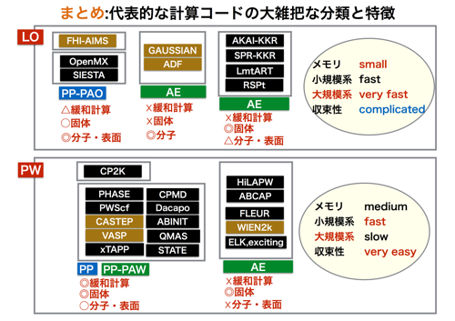
Summary of Calculation Codes

Let me finish with a rather rough summary of calculation codes, admittedly colored by a fair amount of personal judgment and bias. Much of this simply repeats what I have already discussed. From a practical standpoint, I have classified the differences between localized and plane-wave basis sets in terms of memory consumption, computational speed for small and large calculations, and convergence of the electronic states. Within each of those basis-set categories, I have further distinguished pseudopotential and all-electron approaches, and summarized their respective strengths and weaknesses for structural relaxation and for treating bulk solids, molecules, and surfaces.

There are, of course, many gradations between the △ and ○ marks used here, and I am sure quite a few readers will want to object, “No, that’s not right!” I hope you will set those objections aside for the moment and look at the table with a generous spirit. These are deliberately broad tendencies, not hard-and-fast judgments. For beginners, I think the overall impression they convey is not too far removed from practical experience.

Taken as a whole, plane-wave basis sets may look surprisingly versatile. Part of the reason is simply that, in the classification used here, plane-wave basis sets are the only ones rated favorably for structural relaxation, so they inevitably receive a favorable mark in one of the three categories. But in practice, plane waves combined with pseudopotentials really are fairly versatile across the board. They are not necessarily outstanding in any one particular respect—structural relaxation being a notable exception—but the breadth of the field is evident from the development of pseudopotential codes around the world. For molecular systems, on the other hand, quantum-chemistry codes are naturally far superior, with a wealth of analysis capabilities and excellent computational cost-performance. Every approach has advantages and disadvantages. The important thing is to use the right tool for the right job.

1. For example, in calculating XANES spectra, correctly accounting for interactions involving a core hole may require an approach that solves an equation explicitly incorporating two-particle electron correlations, such as the Bethe–Salpeter equation (BSE), rather than solving the DFT–KS equation in its one-electron approximation. ↩

2. Some people mistake the second-variational method for a perturbative approach, but it is not perturbation theory. ↩

3. As a rule of thumb, it is better to regard codes that solve the Dirac equation using four-component spinors, as well as many implementations of the LMTO and KKR methods, as basically employing the MT approximation when treating relativistic effects. There are, of course, exceptions. ↩

4. Most people who measure XAFS spectra—particularly in Japan—probably use an analysis tool called Artemis. Internally, Artemis uses the FEFF calculation code. FEFF actually calculates electronic states within the MT approximation, using the KKR Green’s-function method. This allows it to solve problems extremely quickly and poses no problem at all for EXAFS analysis. Within this approximation, however, calculated XANES spectra for molecules, surfaces, and similar systems often fail to agree with experiment, so caution is required. ↩

5. Finite-difference methods were originally used for macroscopic-scale problems such as fluid dynamics, but more recently they have also been applied to first-principles calculations in codes such as RSPACE. They can handle a broad range of systems, from cluster models to periodic boundary conditions, without being restricted to periodicity. Among other FDM codes, FDMNES, for example, can calculate a wide range of X-ray absorption spectra, from XANES to EXAFS. ↩

6. Of course, some localized bases, such as wavelets, do form a complete basis. ↩

7. Describing d electrons adequately with STOs or GTOs is itself inherently difficult. ↩

8. Naturally, there are also approaches combining localized basis functions with pseudopotentials, so using a localized basis does not necessarily mean that core electrons are always calculated. For example, wavelet bases are generally too coarse to describe core states, and are ordinarily used together with pseudopotentials. In general, however, calculations using STO or GTO bases are usually all-electron calculations. I will summarize the characteristics of individual codes separately. ↩

9. Actually, following the historical development makes these methods easier to understand, so I recommend studying them in that order. There are now many excellent introductory books, including those by R. M. Martin. ↩

10. There are, of course, other all-electron methods applicable to solids. I apologize for leaving them out, but including them would make the discussion considerably longer and more complicated. ↩

11. A representative example is the ghost-band problem encountered when calculating atoms with shallow core states. In fact, introducing local orbitals or explicitly including radial functions orthogonalized to core states has largely resolved the ghost-band problem. Even so, when calculations on unknown materials run into trouble, it is often a linearization problem that brings them to a halt. ↩

12. When calculations disagree with experiment, the cause is often an electron-correlation issue, such as the interaction involving a core hole, rather than a problem with FLAPW itself. On the other hand, FLAPW is fundamentally a linearized band-structure method, so results far from the energy parameters chosen near the Fermi energy are not guaranteed. In this respect it has an intrinsic weakness for calculations covering an extremely broad energy range, as in XAFS. Even so, XANES results often agree reasonably well with experiment. ↩

13. As discussed in the next section, (2)-(C), the PAW method makes it possible to perform calculations involving core states even within a pseudopotential-based framework. ↩

14. If you want to study pseudopotential methods, I think starting with the OPW method makes them easier to understand. ↩

15. Codes using NCPP, USPP, and PAW still coexist today, so strictly speaking I think it is worth understanding the differences among all three. ↩

16. Ultrasoft pseudopotentials do include correction terms. ↩

17. Relaxed-core PAW, in which the pseudopotential used in the calculation itself is reconstructed self-consistently from core-electron states recalculated at each SCF step, should be under development. I hope it eventually emerges from its seemingly eternal alpha stage. ↩

18. The SW-LAPW basis was developed ten years earlier. However, PAW is more commonly discussed as an outgrowth of USPP (and the projectors certainly reflect that lineage), so perhaps only the FLAPW crowd would insist, in a discussion of PAW, that SW-LAPW and PAW have exactly the same form! Still, I think this is a fairly important perspective. ↩

19. Professor Kotani’s documentation provides a detailed comparison of PAW and PMT. His first-principles calculation package, ecalj, is based on the PMT method. ↩

20. Far from being conventional, nobody writes it this way. Be warned: using this notation in public could be embarrassing. ↩

21. PP-PAW is an established notation, although it is somewhat specialized. ↩

22. In the case of pseudopotential methods, there is also the issue of pseudopotential transferability discussed earlier. Whether a supplied pseudopotential will give correct results for the particular structure you wish to calculate is not guaranteed to the same degree for every code—or, indeed, for every pseudopotential used. ↩

23. VASP and CASTEP are both plane-wave-based codes that can perform calculations using USPP and PAW, and are essentially comparable in scope. Although they have developed independently, their origins can be traced back to the same code. I do not know why, but at least in the publicly available version, VASP cannot calculate XANES. Since no pseudopotentials with a core hole are provided, I suspect that the functionality does not exist even as a hidden option. ↩

24. My own experience with AKAI-KKR and SPR-KKR is limited to basic calculations using CPA, so I do not know whether their publicly available versions support XANES calculations including the L edges. To begin with, L-edge calculations involve several intertwined difficulties: spin–orbit coupling, the treatment of excited states, and electron correlation. They are surprisingly difficult. Compared with K-edge calculations, it is much harder to construct a model structure, calculate its spectrum, and discuss the result in a way that can be confidently compared with experiment. Validation against experiment is always necessary. Furthermore, the publicly available versions of these KKR–Green’s-function codes are, of course, subject to the muffin-tin (MT) approximation. This imposes various restrictions on the material systems that can be treated, and calculations often require some ingenuity. ↩

25. Even so, thanks to recent developments in PAW methods using plane-wave bases, it has become possible in many cases to calculate XANES with plane-wave-based codes as well. ↩

26. For example, determining atomic valences. ↩